![[-]](/moniwiki/imgs/plugin/arrup.png "[-]")
![[+]](/moniwiki/imgs/plugin/arrdown.png "[+]")
[edit]
1 왜도(skewness) #
왜도는 분포의 비대칭 정도를 측정하는 척도
skew.f<-function(x)
{
	x<-as.matrix(x)
	n<-nrow(x)
	m<-cov.wt(x)$center
	S<-cov.wt(x,method="ML")$cov
	SI<-solve(S)

	skew<-0
	for(r in 1:n) {
		for(s in 1:n) {
			skew<-skew+(t(x[r,]-m)%*%SI%*%(x[s,]-m))^3
		}
        }
	skew/(n^2)
}
[edit]
2 첨도(kurtosis) #
첨도는 분포의 윗 부분의 평평한 정도를 측정하는 척도
kurtosis.f<-function(x)
{
	x<-as.matrix(x)
	n<-nrow(x)
	m<-cov.wt(x)$center
	S<-cov.wt(x,method="ML")$cov
	SI<-solve(S)


	kurtosis<-0
	for(r in 1:n) {
		kurtosis<-kurtosis+( t(x[r,]-m) %*% SI %*% (x[r,]-m) )^2
	}
	kurtosis/n
}
[edit]
3 정규성 검정 #
normality.f<-function(x,alpha=0.05)
{
	n<-nrow(x)
	p<-ncol(x)
	m<-(p*(p+1)*(p+2))/6
	b1<-skew.f(x)
	p.val<-1-pchisq((n*b1)/6,m)
	cat("Skewness is ",b1,"and P-value is ",p.val,".\n")

	if(p.val < alpha)
		cat("Reject the normality.\n")
	else
		cat("Don't reject the normality.\n")
}
- alpah : 유의수준
- m: 자유도
- p.val: P-Value
다음과 같이 사용한다.
> source("normality.f")
> source("skew.f")
> source("kurtosis.f")
> cork.d <-read.table("cork.d", header=T)
> normality.f(cork.d)
Skewness is  4.476382 and P-value is  0.4036454 .
Don't reject the normality.
[edit]
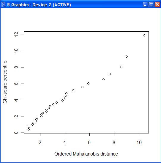
4 카이제곱 그림 #
chiplot.f<-function(x)
{
	n<-nrow(x)
	p<-ncol(x)

	mah<-sort(mahalanobis(x,mean(x),var(x)))
	arr<-seq(from=1/(2*n),length=n,by=1/n);
	chi.per<-qchisq(arr,p)

	plot(mah,chi.per,xlab="Ordered Mahalanobis distance",ylab="Chi-sqare percentile");
}
> source("chiplot.f")
> chiplot.f(cork.d)
[edit]
5 베타그림 #
betaplot.f<-function(x)
{
	n<-nrow(x)
	p<-ncol(x)

	alpha<-(p-2)/(2*p)
	beta<-(n-p-3)/(2*(n-p-1))

	mah<-sort((n/(n-1)^2)*mahalanobis(x,mean(x),var(x)))

	start<-(1-alpha)/(n-alpha-beta+1)
	step<-1/(n-alpha-beta+1)
	arr<-seq(from=start,length=n,by=step)
	beta.per<-qbeta(arr,alpha,beta)

	plot(mah,beta.per,xlab="Ordered b_r",ylab="Beta percentile")
}
> source("betaplot.f")
> betaplot.f(cork.d)
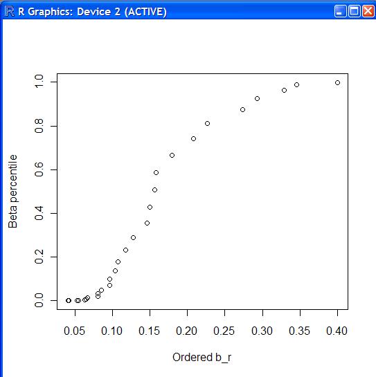
정규성을 가지고 있으나, 꼬리 부분이 약간 짧은 것으로 해석할 수 있다.
[edit]
6 Shapiro 검정 #
- 귀무가설: 정규분포를 따른다. (p-value > 0.05)
- 대립가설: 정규분포를 따르지 않는다. (p-value < 0.05)
> source("rftn.f")
> rad.d <-read.table("rad.d", header=T)
> shapiro.test(rad.d$open)

        Shapiro-Wilk normality test

data:  rad.d$open
W = 0.8292, p-value = 1.977e-05
p-value < 0.05 이므로 정규분포를 따르지 않는다.
[edit]
7 Box-Cox Transformation #
정규 분포에 가깝도록 변환하는 방법
mult.f<-function(lambda, x)
{
	n<-nrow(x)
	p<-ncol(x)
	H<-rep(1,n)%*%t(rep(1,n))/n

	Y<-matrix(0,n,p)
	for(r in 1:n) {
		for(i in 1:p) {
			if( lambda[i] == 0 )
				Y[r,i]<-log(x[r,i])
			else
				Y[r,i]<-(x[r,i]^lambda[i] - 1)/lambda[i]
		}
	}

	Z<-matrix(0,n,p)
	for(i in 1:p) {
		a<-(prod(x[,i]))^((lambda[i]-1)/n)
		Z[,i]<-Y[,i]/a
	}

	log(prod(eigen(t(Z)%*%(diag(n)-H)%*%Z)$values))
}
univ.f<-function(lambda, x)
{
	n<-length(x)
	H<-rep(1,n) %*% t(rep(1,n))/n

	Y<-rep(0,n)
	for(r in 1:n) {
		if( lambda == 0 )
			Y[r]<-log(x[r])
		else
			Y[r]<-(x[r]^lambda-1)/lambda
	}

	Y<-Y/(prod(x)^((lambda-1)/n))
	t(Y)%*%(diag(n)-H)%*%Y
}
boxcox.f<-function(x)
{
	x<-as.matrix(x)
	p<-ncol(x)
	sp<-rep(1,p)

	for(i in 1:p) {
		sp[i]<-nlminb(objective=univ.f,start=sp[i],x=x[,i])$par
	}

	lambda=nlminb(objective=mult.f,start=sp,x=x)$par
	cat("Box-Cox parameters : ",lambda,"\n");

}
> source("boxcox.f")
> source("univ.f")
> source("mult.f")
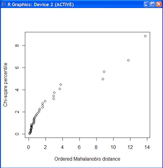
> rad.d <-read.table("rad.d", header=T)
> chiplot.f(rad.d)
> boxcox.f(rad.d)
Box-Cox parameters :  0.1607892 0.1511725
- lamda1 = 0.16
- lamda2 = 0.15
- closed = (closed ^ lamda1 - 1) / lamda1
- open = (open ^ lamda2 - 1) / lamda2
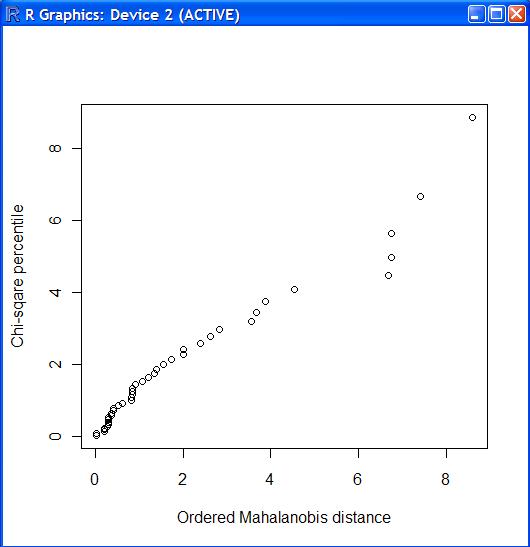
> boxcox_trans.d <- rad.d
> boxcox_trans.d$closed <- (rad.d$closed ^ 0.16 - 1) / 0.16
> boxcox_trans.d$open <- (rad.d$open ^ 0.15 - 1) / 0.15
> boxcox_trans.d
       closed       open
1  -1.6362440 -1.1015160
2  -1.9983371 -2.0210313
3  -1.4996718 -1.1015160
4  -1.9260564 -1.9470281
5  -2.3799621 -1.9470281
6  -1.7980629 -1.8161732
7  -2.0777107 -2.0210313
8  -2.3799621 -1.9470281
9  -2.0777107 -2.0210313
10 -1.9260564 -1.9470281
11 -2.1659062 -2.1928988
...
...

> chiplot.f(boxcox_trans.d)
아니면..
install.packages("TeachingDemos")
library("TeachingDemos")

set.seed(12345)
x <- rnorm(150,1,1)
e <- rnorm(150,0,2)
y <- (.6 *x + 13 + e)^3

hist(y)
hist(bct(y, 0.39))
shapiro.test(bct(y, 0.39))
이렇게.. bct의 2번째 매개변수 lamda를 적절히 조절(0.1~0.9)해 가면서 정규분포로 만든다..